Risk assessment and management is an important aspect in the investment world. The idea is to identify the amount of risk that a portfolio or investments might be exposed to, measure, and, most importantly, develop mitigation measures to keep it low. Value at risk is an important instrument for identifying and measuring risk exposure.
What is Value at Risk?
Value at Risk (VaR) is a financial metric that tries to quantify the level of financial risk within a firm or investment portfolio over a specified period. The metric provides early insight into the amount of loss that one is likely to incur in a given trading position or portfolio over time.

Estimating the amount of risk one is likely to incur is important and a crucial aspect of capital management in the investment world. The estimates are commonly used by investors to make decisions on a set strategy or an investment opportunity.
Calculation
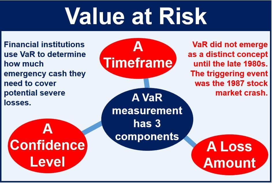
Value at risk is made up of three main components:
- Time period
- Confidence level
- Loss amount, or percentage loss
There are three methods commonly used to evaluate VAR.
Historical method
The historical method assumes that history will always repeat itself in a time in future. Consequently, the VAR evaluation method organizes historical returns putting them in order from the worst to the best.

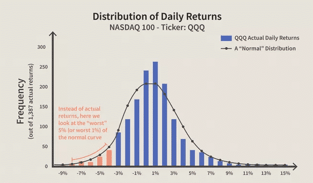
Consider the chart above that shows the Nasdaq 100 ETF with its daily returns. The chart shows more than 250 days when daily returns averaged between 0% and 1%. To the extreme right, it is clear that there were very few days where the ETF daily returns averaged 13%, probably one day, to be specific.
The bars to the left show the amount of risk exposure that the ETF generated losses amounting to risk. The red bars show losses of between 4% and 8%. In this case, we can say that with 95% confidence that daily loss in any given trading day is unlikely to exceed 4%. Conversely, one can expect with 95% confidence that the daily gain will always exceed -4%
With the historical method, the data is used to ascertain the prospects of generating losses and the amount of loss one is likely to incur. For the example above, it is clear that any investment involving the Nasdaq ETF will always be susceptible to a maximum loss of -4% on any given day.
However, the model does not express with certainty the amount of loss one is likely to incur. Instead, it provides a probability from which investment decisions can be made.
Variance Covariance method
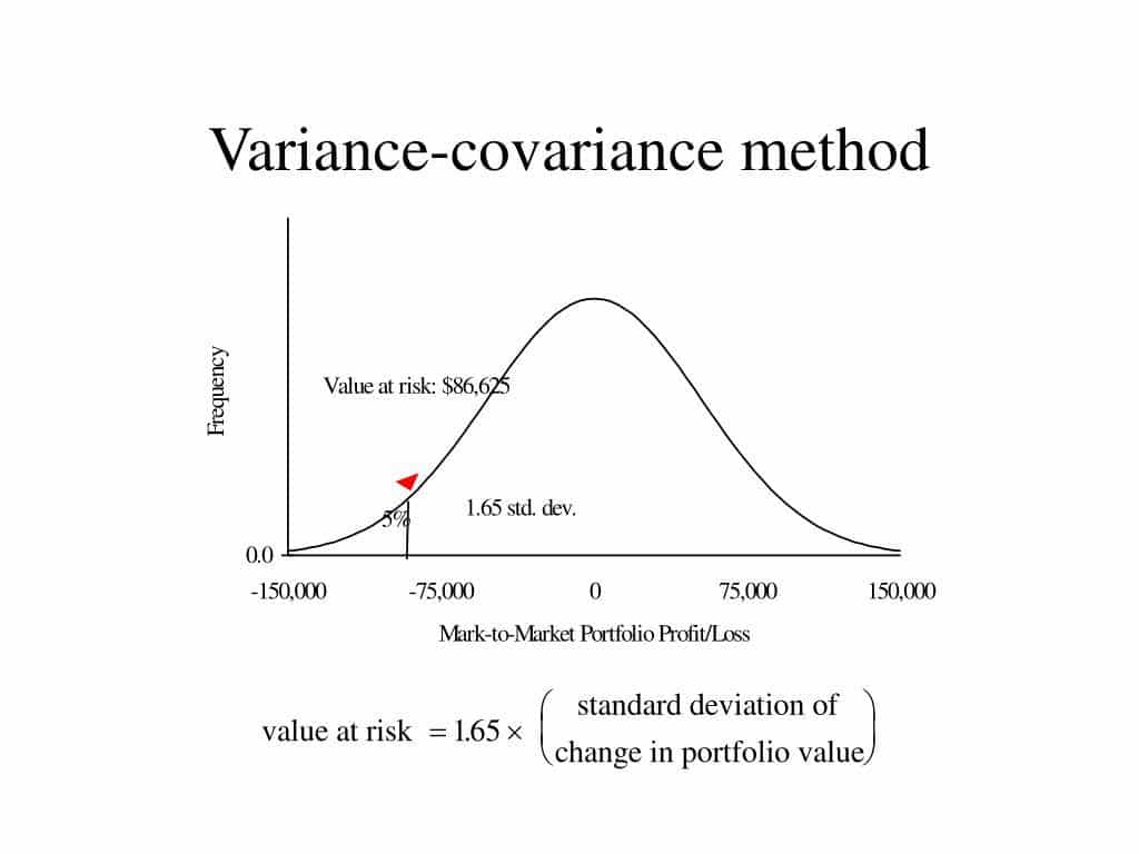
The VAR calculation method assumes that investment returns will always be distributed. In this case, the method entails estimating the expected average return and a standard deviation from the returns. Conversely, a normal curve is plotted against the actual return data.

The use of a normal curve makes it easy to know where the worst 5% and 1% will lie. In the histogram above, the standard deviation of the QQQ ETF was 2.64%. Consequently, the average daily return happened close to zero.
Monte Carlo simulation
The Monte Carlo simulation model entails envisioning future returns on an investment portfolio and running hypothetical trials. The model relies on a software program to generate the distribution of returns on a security or portfolio.
The returns are generated based on the inputs provided regarding the historical return and standard deviation of the asset under study. The fact that the model generates trials randomly means it does not tell anything concrete about the underlying methodology.
After the simulation on the QQQ ETF, two outcomes came out clear of between -15% and -20%, with three outcomes indicating potential losses of between -20% and 25%. With these results, it is clear that with 95% confidence in the QQQ ETF, one cannot expect to lose more than 15% in any given month.
Why Value at risk?
Value at risk stands out as an important investment metric as it provides a clear outline of the market risks one should expect. The measure can be used to measure the risk of asset classes’ exhibiting different risk characteristics.
The measure is often used in the risk budgeting process where management allocates VaR across divisions. In return, the managers are tasked with the responsibility of maximizing the returns based on the VaR allocated. Conversely, the measure is used to ascertain the performance of various units based on the allocated VAR.
In addition, Value at risk is an easy-to-understand financial metric as it indicates the extent of risk in a given portfolio. It is measured in either price units or percentages, making it easy to understand and interpret.
Limitations
It can be extremely difficult to calculate the value at risk when dealing with large portfolios. In this case, one will have to calculate the risk and return of each asset. The greater the diversity of the assets involved, the more calculations one will take.
The different methods used in calculating VAR can also prove to be a big challenge. For starters, each method can provide a different outcome making it extremely difficult to understand the risk profile of each asset.
The assumptions made in its calculations also pose significant risks, given that one might end up with a risk profile that is not accurate. Whenever the assumptions are not valid, then the likelihood of ending up with an invalid VaR is usually high.
Final thoughts
Value at risk is an important risk management measure used by portfolio managers worldwide. The measure makes it easy to have a clear idea of the maximum loss one is likely to incur in an investment over a given period. While VAR’s advantages in risk measurement outweigh its disadvantages, it is important to consider some of the limitations of the measures.


